
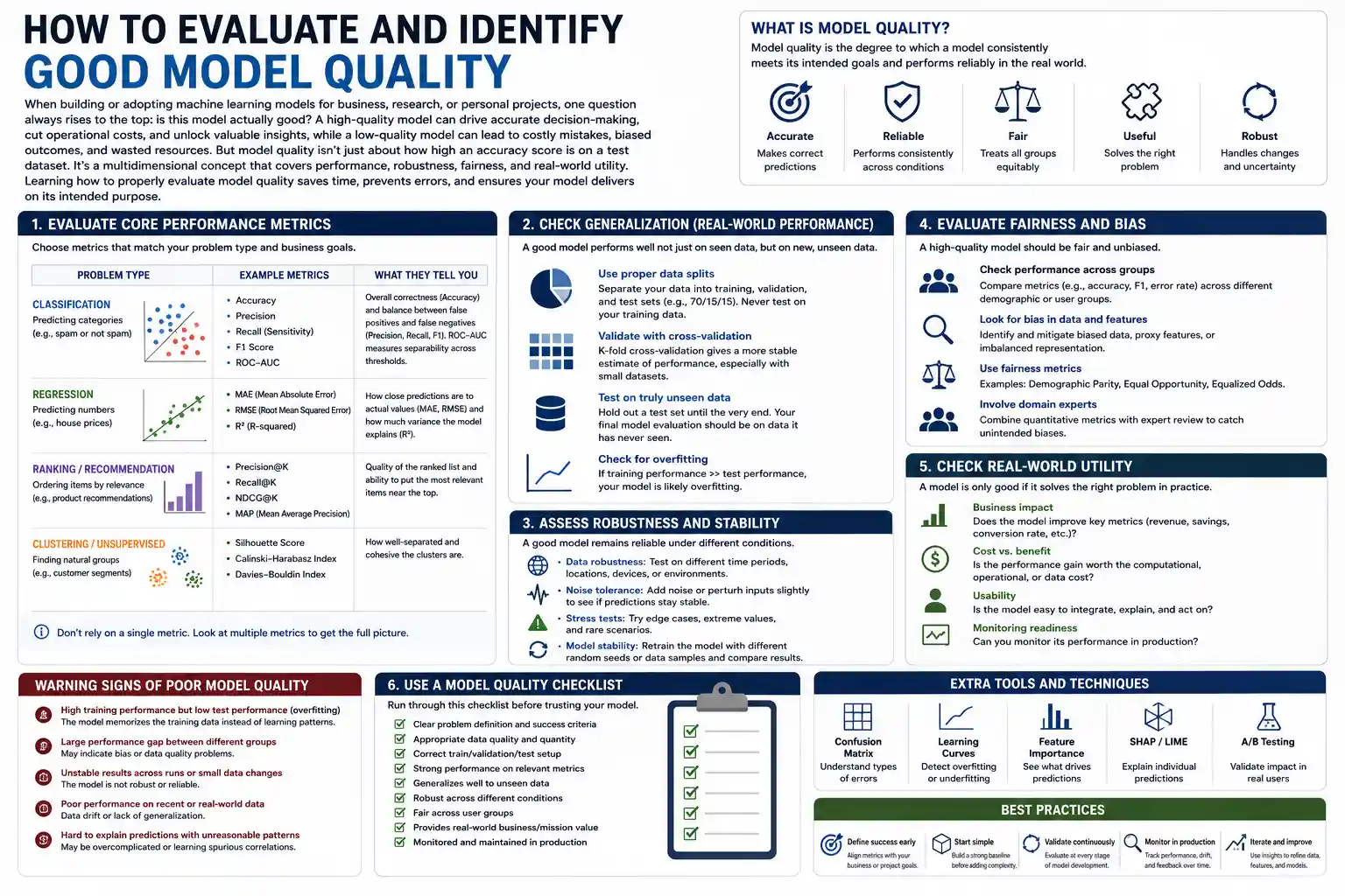
When building or adopting machine learning models for business, research, or personal projects, one question always rises to the top: is this model actually good? A high-quality model can drive accurate decision-making, cut operational costs, and unlock valuable insights, while a low-quality model can lead to costly mistakes, biased outcomes, and wasted resources. But model quality isn’t just about how high an accuracy score is on a test dataset. It’s a multidimensional concept that covers performance, robustness, fairness, and real-world utility. Learning how to properly evaluate model quality saves time, prevents errors, and ensures your model delivers on its intended purpose.
Core Performance Metrics: Beyond Overall Accuracy
The first step in evaluating model quality is measuring core predictive performance, but many people make the mistake of relying solely on overall accuracy to judge a model. Accuracy—the percentage of correct predictions out of total predictions—can be misleading, especially for imbalanced datasets, where one class makes up the vast majority of observations. For example, a model that predicts no fraud in 10,000 credit card transactions will be 99% accurate if only 1% of transactions are fraudulent, but it’s completely useless for catching actual fraud. To get a full picture of performance, you need to look beyond overall accuracy at more granular metrics tailored to your use case.
Key Classification Metrics for Categorical Outcomes
For classification models that sort inputs into discrete categories, there are several core metrics that reveal how well the model performs across different classes. Precision measures how many of the model’s positive predictions are actually correct—this is critical for use cases where false positives are costly, like spam detection: marking a legitimate email as spam (a false positive) is more harmful than letting one spam email through. Recall (also called sensitivity) measures how many of the actual positive cases the model caught, which is critical for medical diagnostics: missing a case of cancer (a false negative) is far more dangerous than incorrectly flagging a healthy patient. The F1-score is the harmonic mean of precision and recall, giving a single score that balances both metrics. For multi-class classification, you can also look at per-class accuracy and macro vs. micro averaged scores to spot if the model performs well on common classes but poorly on rare ones.
Key Regression Metrics for Continuous Outcomes
For regression models that predict continuous values, like housing prices or monthly sales, the most common metrics are mean absolute error (MAE), mean squared error (MSE), and root mean squared error (RMSE). MAE measures the average absolute difference between predicted and actual values, and it’s easy to interpret because it’s in the same unit as your outcome: an MAE of $12,000 for housing price predictions means the average prediction is off by $12,000. MSE penalizes larger errors more heavily than MAE, because it squares the difference between predictions and actuals, making it useful when large mistakes are especially costly. RMSE is just the square root of MSE, putting it back into the original unit of measurement for easier interpretation. It’s also helpful to look at R-squared, which measures how much variance in the outcome your model explains compared to a simple baseline prediction of the average value. An R-squared close to 1 means your model explains most of the variance, while a negative R-squared means your model is worse than just predicting the average.
It’s also important to compare your model’s performance to a meaningful baseline, not just look at the raw metric. A model with 85% accuracy sounds impressive, but if a simple rule-based model already gets 83% accuracy, the extra complexity of your machine learning model isn’t worth it. Always benchmark against the simplest possible solution to verify that your model adds real value.
Evaluating Generalization: Avoiding Overfitting and Underfitting
One of the biggest threats to model quality is poor generalization: a model that performs great on your test dataset but fails completely when deployed on new, unseen data. This usually happens because of overfitting, where the model learns random noise and idiosyncrasies in your training data instead of the underlying pattern that applies to new data. For example, if you’re training a model to identify cats from photos, and all the cats in your training dataset happen to be on grass, an overfit model might learn that “green pixels in the background” means the photo contains a cat. It will get 100% accuracy on your training set, but fail when a cat is photographed on a couch. The opposite problem, underfitting, happens when the model is too simple to capture the underlying pattern, leading to poor performance on both training and test data.
Proper Cross-Validation for Reliable Generalization Estimates
To accurately measure how well your model generalizes, you need a solid validation strategy. Holdout validation, where you split your data into separate training, validation, and test sets, is a good starting point, but it can give variable results depending on how you split the data. For a more reliable estimate of generalization performance, k-fold cross-validation is the industry standard.
The process for k-fold cross-validation is straightforward:
- Shuffle your full dataset randomly, then split it into k equal-sized groups (folds), typically 5 or 10.
- Hold out one fold as a test set, and train your model on the remaining k-1 folds.
- Evaluate the trained model on the held-out fold and record the performance metric.
- Repeat this process until every fold has been held out once as the test set.
- Average the performance across all k runs to get an overall estimate of generalization.
If you have a very large dataset, stratified k-fold cross-validation is even better for imbalanced datasets, because it ensures each fold has roughly the same distribution of classes as the full dataset. This prevents you from getting a fold that has no examples of a rare class, which would skew your performance estimate.
Learning Curves to Diagnose Overfitting and Underfitting
A learning curve is a simple but powerful tool to diagnose model quality and understand whether you need more data or a more complex model. It plots model performance (like accuracy or error) on both the training set and the cross-validation set as the size of the training dataset increases. The shape of the curve tells you a lot about the model’s generalization:
- If training error is low and cross-validation error is much higher than training error, you have overfitting. The gap between the two curves is the overfitting gap. To fix this, you can try adding more training data, using regularization to reduce model complexity, or simplifying your model architecture.
- If both training error and cross-validation error are high, and the gap between them is small, you have underfitting. This means your model is too simple to capture the pattern in the data. To fix this, you can try adding more features, increasing model complexity, or using a different model architecture.
- If both training error and cross-validation error are low, and the gap between them is small, your model has good generalization and high quality.
By using cross-validation and learning curves, you can avoid the common mistake of thinking a model is high-quality just because it performs well on a single held-out test set. A truly high-quality model performs consistently across different subsets of your data, not just one lucky split.
Robustness and Reliability: Does the Model Hold Up Under Real-World Conditions?
Predictive performance and generalization on held-out data are important, but they don’t tell the whole story about model quality. A model can have great cross-validation accuracy but still fail in production because it’s not robust to small changes in input data or unexpected edge cases. High-quality models are reliable: they perform consistently even when real-world conditions don’t match the conditions they were trained on.
Sensitivity to Input Changes and Adversarial Perturbations
One way to test robustness is to measure how sensitive the model’s predictions are to small, meaningless changes in input data. For example, in an image classification model, adding tiny amounts of random noise to a photo of a dog shouldn’t change the model’s prediction. If the model suddenly calls the dog a truck after adding almost imperceptible noise, it’s not robust. For tabular data, you can test robustness by slightly changing the values of input features within their normal range and seeing if predictions change dramatically. For example, a credit scoring model that suddenly approves a high-risk application just because the applicant’s annual income is increased by $100 is low-quality, because it’s over-reliant on one small input change.
For high-stakes applications like autonomous driving or facial recognition, it’s also important to test for adversarial perturbations: intentionally crafted small changes to input that trick the model into making a mistake. Even if these changes are invisible to humans, they can cause low-quality models to fail catastrophically. A high-quality model will be resistant to these common types of attacks.
Handling Distribution Shift Over Time
Another major threat to real-world model quality is distribution shift, which happens when the statistical properties of the input data or the relationship between inputs and outputs change over time after the model is deployed. For example, a fraud detection model trained on pre-pandemic spending patterns will perform poorly in 2025, because consumer behavior has shifted dramatically. A demand forecasting model trained on pre-COVID retail data will fail to predict the sudden changes in online shopping behavior after 2020.
All models are wrong, but some are useful in the real world—usefulness depends on how well they adapt to change, not just how accurate they were on a training set collected five years ago.
To test a model’s ability to handle distribution shift, you can do what’s called out-of-time validation: train the model on data from one time period, and test it on data from a later time period. If the model still performs well on the newer data, it’s much higher quality than a model that only performs well on random cross-validation splits that mix data from different time periods. For example, if you’re building a model to predict customer churn in 2024, you can train on 2021 data and test on 2022 data, then train on 2022 data and test on 2023 data, to see how well it performs as customer behavior changes. This gives you a much more realistic estimate of how it will perform when deployed than random cross-validation.
You can also test how the model handles missing data, which is almost inevitable in real-world deployments. A high-quality model will have built-in handling for missing values and won’t produce extreme or incorrect predictions when some features are missing. A low-quality model will fail completely if even one input feature is missing, which makes it unreliable for production.
Fairness and Ethical Quality: Avoiding Harmful Bias
In recent years, it’s become clear that model quality isn’t just about performance and reliability—it’s also about fairness. A model that has high predictive accuracy but systematically discriminates against protected groups is low quality, because it causes harm and often doesn’t comply with regulatory requirements like the EU’s AI Act or the US Equal Credit Opportunity Act. Evaluating fairness is a critical part of assessing model quality for any high-stakes application, from hiring to lending to criminal justice.
Key Fairness Metrics to Measure Disparate Impact
There are several common metrics used to evaluate whether a model has unfair bias across different demographic groups. For classification models, equalized odds requires that the model has the same true positive rate and false positive rate across all protected groups. For example, a loan approval model should have the same false rejection rate for qualified applicants of different races: if qualified Black applicants are rejected at twice the rate of qualified white applicants, the model fails equalized odds and is low quality. Demographic parity requires that the model approves roughly the same percentage of applicants from each group, though this can sometimes conflict with overall accuracy. Equal opportunity is a slightly relaxed version of equalized odds that only requires the same true positive rate across groups, which is often more practical for real-world use cases.
To evaluate fairness, you need to disaggregate your performance metrics by group. Instead of just looking at overall accuracy or recall, calculate recall, false positive rate, and precision separately for each protected group (like gender, race, age, or disability status). If the model performs substantially worse on one group than others, that’s a red flag that the model is low quality, even if overall performance is good.
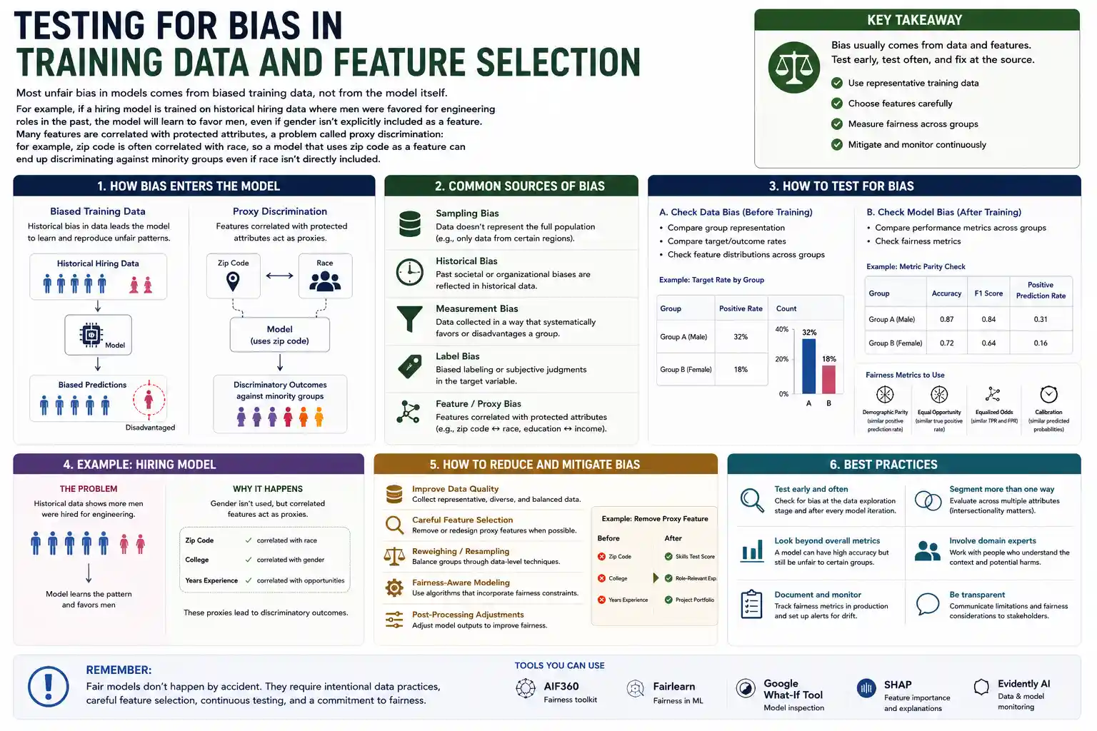
Most unfair bias in models comes from biased training data, not from the model itself. For example, if a hiring model is trained on historical hiring data where men were favored for engineering roles in the past, the model will learn to favor men, even if gender isn’t explicitly included as a feature. Many features are correlated with protected attributes, a problem called proxy discrimination: for example, zip code is often correlated with race, so a model that uses zip code as a feature can end up discriminating against minority groups even if race isn’t directly included.
To check for this type of bias, you can measure the correlation between your input features and protected attributes. If a feature is highly correlated with a protected attribute, ask yourself whether that feature is actually necessary for prediction, or whether it’s just capturing historical bias. You can also use bias mitigation techniques like reweighting training examples or adversarial debiasing to reduce disparate impact, but the first step is always measuring it to identify the problem.
Fairness isn’t always a binary “fair or unfair” outcome, but it’s an important component of overall model quality. A model that causes harm to vulnerable groups is not a high-quality model, no matter how accurate it is.
Operational and Business Quality: Does the Model Meet Real-World Needs?
Finally, model quality depends on how well the model meets your operational and business needs, beyond technical performance metrics. A technically perfect model that can’t be deployed, is too slow to run, or doesn’t answer the question you need answered is low quality for your use case. This is often an overlooked aspect of model evaluation, but it’s critical for real-world adoption.
Operational Complexity and Maintainability
High-quality models are maintainable and fit into your existing infrastructure. If you’re a small business with limited engineering resources, a complex deep learning model that requires specialized hardware to run and a team of data scientists to maintain is lower quality for your needs than a simpler gradient boosting model that runs on your existing servers and is easy to update. Some questions to ask when evaluating operational quality include:
- How much time and resources does it take to retrain the model with new data?
- Can your existing engineering team debug the model if it makes a mistake?
- Does the model’s inference time meet your latency requirements? A recommendation model that takes 2 seconds to load a page will hurt user experience, even if it’s more accurate than a faster, slightly less accurate model.
- How much storage and compute does the model require, and does that fit your budget?
For example, a self-driving car model needs to make predictions in milliseconds to be safe. A model that gets 99% accuracy but takes 500 milliseconds to make a prediction is too slow for use, making it low quality for that application. On the other hand, a model that’s used for daily batch forecasting of sales can tolerate longer run times, so complexity is less of an issue.
Interpretability and Stakeholder Trust
For many use cases, especially high-stakes ones, stakeholders need to understand why the model makes a certain prediction. A credit lender is required by law to explain to an applicant why their loan was rejected, and doctors need to understand why a model recommended a certain treatment to trust it. A black box model that makes accurate predictions but can’t explain its decisions is lower quality for these use cases than a slightly less accurate but interpretable model.
You can evaluate interpretability by checking whether you can answer simple questions about the model’s behavior: Which features are the most important for predictions? Does the relationship between a feature and the prediction make logical sense? For example, a credit scoring model that says higher annual income leads to lower credit risk makes logical sense, while a model that says higher income leads to higher credit risk is suspicious, even if it has high accuracy on test data. Tools like SHAP and LIME can help you interpret black box models by showing how each feature contributes to individual predictions, but inherently interpretable models like linear regression or decision trees are often easier to explain to non-technical stakeholders.
Ultimately, a model that no one trusts will never be used, so even the most technically accurate model is low quality if it doesn’t build trust with the people who rely on it.
Conclusion
Evaluating model quality is a multidimensional process that goes far beyond checking a single accuracy score. A high-quality model has strong performance on relevant metrics, generalizes well to new data, is robust to real-world changes and edge cases, is fair across different groups of people, and fits your operational and business needs. By following a structured evaluation process that checks each of these dimensions, you can avoid the common mistake of deploying a model that looks great on paper but fails in practice. Whether you’re building a model for a small business project or a large enterprise deployment, taking the time to properly assess each aspect of model quality will save you time, money, and harm down the line. The best model isn’t always the one with the highest accuracy—it’s the one that meets all of your needs, for the people who will actually use it.